Creates an empirical distribution object from a sample.
Assumes iid. samples. with_params should not be used with this
distribution because estimation of the relevant indicators happens during
construction.
Arguments
- sample
Sample to build the empirical distribution from
- positive
Is the underlying distribution known to be positive? This will effect the density estimation procedure.
positive = FALSEuses a kernel density estimate produced bydensity(),positive = TRUEuses a log-kernel density estimate produced bylogKDE::logdensity_fft(). The latter can improve density estimation near zero.- bw
Bandwidth parameter for density estimation. Passed to the density estimation function selected by
positive.
Details
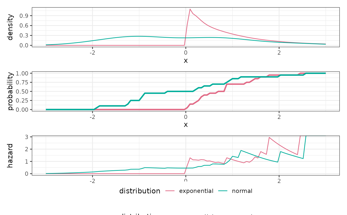
sample()samples iid. fromsample. This approach is similar to bootstrapping.density()evaluates a kernel density estimate, approximating with zero outside of the known support. This estimate is either obtained using stats::density or logKDE::logdensity_fft, depending onpositive.probability()evaluates the empirical cumulative density function obtained by stats::ecdf.quantile()evaluates the empirical quantiles using stats::quantilehazard()estimates the hazard rate using the density estimate and the empirical cumulative density function:h(t) = df(t) / (1 - cdf(t)).
See also
Other Distributions:
Distribution,
dist_bdegp(),
dist_beta(),
dist_binomial(),
dist_blended(),
dist_dirac(),
dist_discrete(),
dist_erlangmix(),
dist_exponential(),
dist_gamma(),
dist_genpareto(),
dist_lognormal(),
dist_mixture(),
dist_negbinomial(),
dist_normal(),
dist_pareto(),
dist_poisson(),
dist_translate(),
dist_trunc(),
dist_uniform(),
dist_weibull()
Examples
x <- rexp(20, rate = 1)
dx <- dist_empirical(sample = x, positive = TRUE)

y <- rnorm(20)
dy <- dist_empirical(sample = y)

plot_distributions(
  exponential = dx,
  normal = dy,
  .x = seq(-3, 3, length.out = 100)
)
